Querying Time Series in Postgresql
May 8, 2014 - Portland, OR
This post covers some of the features which make Postgresql a fun and effective database system for storing and analyzing time series: date functions, window functions, and series generating functions.
What are time series?
In a computation context, a time series is a sequence of measurements taken at discrete time intervals. Measurements can be taken every second, hour, day, or other arbitrary interval. The code below will generate some time series data on the activity in a Postgresql cluster by sampling pg_stat_activity every 10 seconds for 100 seconds.
-- add a table to store some time series data
create table activity_tseries (measured_at timestamptz, activity_count int);

-- add a pl function to collect counts of active queries at 10 second intervals
create or replace function collect_activity() returns void AS $$
  begin
    for i in 1..10 loop
      insert into activity_tseries (measured_at, activity_count) values
        (clock_timestamp(), (select count(*) from pg_stat_activity where state <> 'idle'));
      perform pg_sleep(10);
    end loop;
  end;
$$ language plpgsql;

-- collect the data
select collect_activity();
Consider the output, a sequence of activity measurements at 10 second intervals. Note the selection of a timestamp and an associated metric.
postgres=# select measured_at, activity_count from activity_tseries;
          measured_at          | activity_count
-------------------------------+----------------
 2014-05-07 18:22:09.655861-07 |             11
 2014-05-07 18:22:19.664114-07 |             10
 2014-05-07 18:22:29.674501-07 |              3
 2014-05-07 18:22:39.676574-07 |              9
 2014-05-07 18:22:49.686977-07 |              5
 2014-05-07 18:22:59.697342-07 |              6
 2014-05-07 18:23:09.707722-07 |              4
 2014-05-07 18:23:19.70827-07  |              6
 2014-05-07 18:23:29.718338-07 |              4
 2014-05-07 18:23:39.719099-07 |              2
(10 rows)
Continuous, Discrete, and Granularity – Changes Over Time Domain
It’s kind of difficult to look at a large number of data points and attribute meaning. So it’s common to ask questions like “how many activities were observed by hour?” Maybe that would highlight a trend or pattern in activity.
This is where date_trunc comes into the picture. Used with a sum aggregate we can easily count activities by minutes.
postgres=# select date_trunc('minute', measured_at) as mins, sum(activity_count)
              from activity_tseries
              group by date_trunc('minute', measured_at)
              order by date_trunc('minute', measured_at) asc;

          mins          | sum
------------------------+-----
 2014-05-07 18:22:00-07 |  44
 2014-05-07 18:23:00-07 |  16
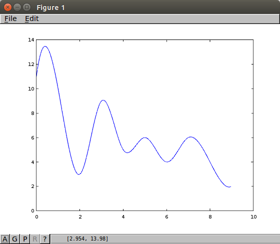
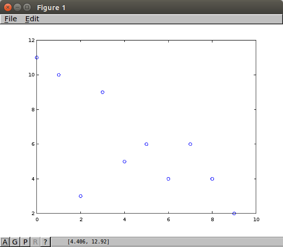
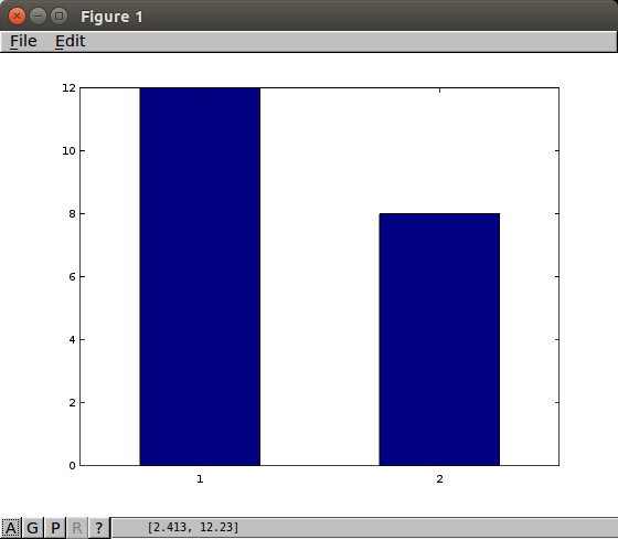
Representations of the a theoretical continuous sample, actual samples, the aggregated samples from this section are pictured below.
 |
 |
 |
Quick Practical Example
Before moving on to some more interesting features, here’s a quick example that will be widely applicable and that will set the stage for the next section. Lets consider counting the number of new user records by day based on a created_at timestamp. These are some actual numbers from The Drift, in case you are curious about the adoption of a free Android application in its first months:
postgres=# select date_trunc('day', created_at) as day, count(*)
              from users
              group by date_trunc('day', created_at)
              order by date_trunc('day', created_at) asc;

     date_trunc      | count
---------------------+-------
 2014-01-05 00:00:00 |     1
 2014-01-13 00:00:00 |     1
 2014-01-14 00:00:00 |     1
 2014-01-15 00:00:00 |     1
 2014-01-16 00:00:00 |     1
 2014-02-10 00:00:00 |     1
 2014-02-13 00:00:00 |     1
 2014-02-14 00:00:00 |     2
 2014-02-18 00:00:00 |     1
 2014-02-19 00:00:00 |     2
 2014-02-21 00:00:00 |     1
 2014-02-23 00:00:00 |     2
 2014-02-24 00:00:00 |     1
 2014-03-02 00:00:00 |     1
 2014-03-03 00:00:00 |     1
 2014-03-06 00:00:00 |     3
 2014-03-09 00:00:00 |     2
...
Interval Filling
Let’s say we wanted to reason about the rate of adoption from the above result set, or plot this data in a simple plotting library. We might have a problem. There are numerous gaps in the data where there were no results, e.g. from January 5th and January 13th. The library may not support parsing date strings and managing the time axis properly.
A straightforward technique to solve this problem is to outer join a result set from the generate_series function.
postgres=# with filled_dates as (
  select day, 0 as blank_count from
    generate_series('2014-01-01 00:00'::timestamptz, current_date::timestamptz, '1 day')
      as day
),
signup_counts as (
  select date_trunc('day', created_at) as day, count(*) as signups
    from users
  group by date_trunc('day', created_at)
)
select filled_dates.day,
       coalesce(signup_counts.signups, filled_dates.blank_count) as signups
  from filled_dates
    left outer join signup_counts on signup_counts.day = filled_dates.day
  order by filled_dates.day;

          day           | signups
------------------------+---------
 2014-01-01 00:00:00-07 |       0
 2014-01-02 00:00:00-07 |       0
 2014-01-03 00:00:00-07 |       0
 2014-01-04 00:00:00-07 |       0
 2014-01-05 00:00:00-07 |       1
 2014-01-06 00:00:00-07 |       0
 2014-01-07 00:00:00-07 |       0
 2014-01-08 00:00:00-07 |       0
 2014-01-09 00:00:00-07 |       0
 2014-01-10 00:00:00-07 |       0
 2014-01-11 00:00:00-07 |       0
 2014-01-12 00:00:00-07 |       0
 2014-01-13 00:00:00-07 |       1
 2014-01-14 00:00:00-07 |       1
 2014-01-15 00:00:00-07 |       1
 2014-01-16 00:00:00-07 |       1
 2014-01-17 00:00:00-07 |       0
Finite Difference (Discrete Derivative)
Here’s an interesting case for estimating a time series for the transactions/second being processed by a Postgresql cluster. This is a real problem that came up when building Relational Systems.
We start by collecting familiar time series data into a metrics table. In this case we collect a timestamp associated with the result of the txid_current function.
          measured_at          | current_tx_id
-------------------------------+---------------
 2014-05-03 13:20:46.797304-07 |       1732896
 2014-05-03 13:21:05.012321-07 |       1732923
 2014-05-03 13:21:20.05257-07  |       1732945
 2014-05-03 13:21:35.069332-07 |       1732962
 2014-05-03 13:21:50.102453-07 |       1732991
 2014-05-03 13:22:05.127961-07 |       1733002
 2014-05-03 13:22:20.162577-07 |       1733023
 2014-05-03 13:22:35.189161-07 |       1733034
 2014-05-03 13:22:50.21059-07  |       1733056
 2014-05-03 13:23:20.319999-07 |       1733070
 2014-05-03 13:23:47.909198-07 |       1734933
Ignoring wraparound cases for simplicity, the goal is to query this data for a result set which represents the familiar formula:
\[\frac{\text{txid_current}_{n} - \text{txid_current}_{n-1}}{\Delta t_{sec}} \approx \frac{transactions}{second}\]And, fortunately, this is simple with the amazing feature that is window functions.
postgres=# select measured_at,
              (current_tx_id - lag(current_tx_id, 1) over w) /
                extract( epoch from  (measured_at - lag(measured_at, 1) over w))::numeric
                  as tx_sec
            from heartbeats
              window w as (order by measured_at)
            order by measured_at desc;

          measured_at          |         tx_sec
-------------------------------+------------------------
 2014-05-04 13:02:56.456229-07 |     1.4642749200123185
 2014-05-04 13:02:41.431728-07 | 0.79921937579501514887
 2014-05-04 13:02:26.417077-07 |     1.4637795079651562
 2014-05-04 13:02:11.387491-07 | 0.79917248353238499975
 2014-05-04 13:01:56.371959-07 |     1.4634836872125585
 2014-05-04 13:01:41.339335-07 | 0.79888332089405429091
 2014-05-04 13:01:26.318368-07 |     1.4639291192137370
 2014-05-04 13:01:11.290318-07 | 0.79880897581705676836
 2014-05-04 13:00:56.267953-07 |    26.7313182385336655
 2014-05-04 13:00:40.743092-07 | 0.49860550013721623364
 2014-05-04 13:00:10.659188-07 |     2.3291032160723028
Window functions allow you to reference records in a window, which is a set of records which have a relationship to the current row. In the example above, the query uses the lag function which returns a value from a row offset before the current row. The window for this query is ordered by the timestamp measured at. Because a lag of 1 references the previous sample of txid_current() the tx_sec field matches the desired formula.
Window functions are remarkably powerful as you can apply aggregates over windows.
Below is a plot based on this query showing what happens when running pgbench -T 100 -c 20 on a commodity desktop.

Final Remarks
The examples illustrate how easy and effective Postgresql can be for querying time series data with date functions, window functions, and series generating functions. There are many more great tools for this type of querying that I hope to explore in future posts.